Statistics Calculators
SUBEDI CALCnew window | DESMOS Calculatornew window | STATKEYnew window | LibreTEXT Calculatorsnew window
- Geogebra Statistical Distributions and Testsnew window
- Rossman/Chance Applet Collectionnew window
- Statology Calculatorsnew window
- Statistics Calculators by David Lanenew window
- Calculators by Matt Bognarnew window
Generate Random Numbers
Random Number Generatornew window
This calculator allows you to generate random numbers between a start and end value. Option to allow duplicates is available.
Calculator Screenshot

Generating Random Values
Generate a random value sampled uniformly from the interval [0,1).
random()
Generate a list of n random values sampled uniformly from the interval [0,1).
random(n)
Generate a list of n random values sampled uniformly from the interval [0,1), using seed.
random(n, seed)

Generating Random Numbersnew window
Generate a random number between 0 and 1.

[MATH] > PROB
Select 1:rand and ENTER
Generate n random number between 0 and 1.

[MATH] > PROB
Select 1:rand followed by ( n ) and ENTER
Generate n random number between lower and upper values.

[MATH] > PROB
Select 5:randInt and enter lower, upper, and the number of random values to generate. Select Paste
and press ENTER. Press ENTER again.
NOTE: For older operating systems, enter as
randInt(1, 100, 5)
Generating Random Numbers (MS EXCEL, GOOGLE SHEETS, etc.)
=RAND()
Generate a random integer between two values, inclusive.
=RANDBETWEEN(low, high)
 and Randbetween()")
Descriptive Statistics
Calculate one variable summary statistics for raw data or data presented in a frequency table.

Calculator Screenshot showing calculation for data frequency table. For raw data, only the first column will show.
Weighted Mean and Expected Value Calculatornew window
Calculate weighted means from supplied data. For expected value, ensure the probabilities
sum to 1.

DESMOS: Summary Statistics
Enter your raw data values as a comma separated list inside square brackets. Give the list a name so that the list can be referenced later for calculations. Example: L= [25,36,45,25,-6,25,48]
Desmos General Statistical Functionsnew window
Finding a 5-Number Summary using Desmos

One Variable Statistics Calculatornew window
Enter data values in the text entry box. Separate values with commas. See screenshot below:

Descriptive Statistics for One Quantitative Variablenew window
On the main StatKey page, click on One Quantitative Variable under Descriptive Statistics and Graphs.
Enter your data by clicking on EDIT DATA button.
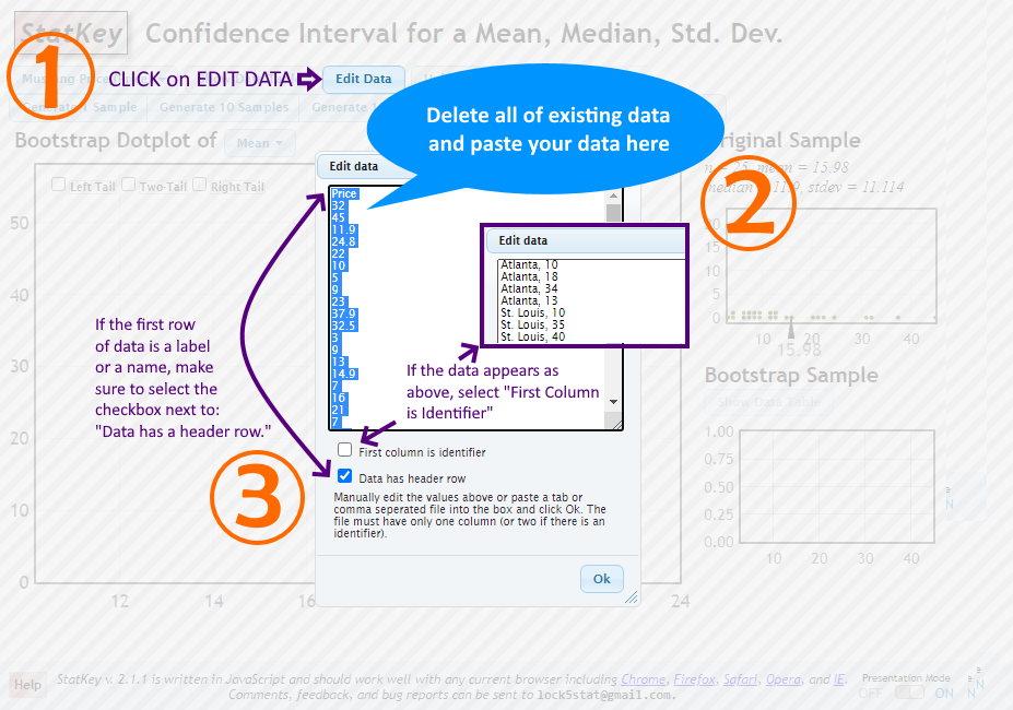
Manually edit the values or paste a tab or comma seperated file into the box and click Ok.
If updating a data file, ensure there's only one column (or two if there is an identifier).
After entering your data, you will see something similar to the image below:

Descriptive Statistics
In addition to the summary statistics, StatKey also can nicely graph supplied data. Enter your data. For help with data entry, see the Edit Data section of Statkey tab inside Summary Statistics.
Once data values are entered, the default graph is dislayed. Choose the options below for various graph types and summaries.
- One Quantitative Variablenew window [Dotplot, Histogram, Box plot]
- One Categorical Variablenew window [Bar Graph]
- One Quantitative and one Categorical Variablenew window [Dotplot, Histogram, Box plot]
- Two Categorical Variablesnew window [Bar Graph]
- Two Quantitative Variablesnew window [Scatterplot]


Boxplot and Five-Number Summary (TI-83 & TI-84)
Normal and Student-t distributions
Probability Distributions (Z, t)new window
Calculate cdf and inverse for Normal and Student-t distributions. For entered values, the results displayed are from Desmos. Desmos input entries are also displayed to help you use Desmos Graphing Calculator directly if you wish.
")
CDF and InverseCDF
On the StatKey Home Pagenew window main page, select either Normal or t for Theoretical Distributions row.
For normal distribution, you can change the mean and the standard deviation values by clicking on [ Edit Parameters ] button.
For Student-t, enter degrees of freedom (df), which you can change later as needed by clicking on [ Edit Parameters ] button.
Select Left Tail, Right Tail, or Two Tail and enter either an area/proportion/probability or values (x or z). Results will automatically be shown.
Screenshot showing Normal distribution example with two tails.

Compute r, r2, and the Linear Regression equation
LINEAR REGRESSION and CORRELATIONnew window
Make sure to view the Regression Tournew window first before using Desmos for regressions.
Screenshot of Desmos Regression Entry

For linear regression, follow the Two Quantitative Variablesnew window link under Descriptive Statistics and Graphs on the main StatKey page. This is the same one from Descriptive statistics above.
Enter your data values by clicking on the EDIT Data button. Your summary statistics should automatically show.
Use the options to switch variables or Show Regression Line as necessary.
Screenshot of Descriptive Statistics for Two Quantitative Variables with regression equation shown.

Linear Regression on a TI-83 and TI-84
One sample and Two samples
Confidence Interval for Proportionsnew window
Calculate confidence interval (CI) for proportion for both one or two sample cases. CI is given in ± notation. Margin of Error is also shown.

CONFIDENCE INTERVAL for proportions Calculatornew window
Enter sample size, n, the number of successes, x, and the confidence level, CL (in decimal). Press calculte to reveal the lower and upper bounds of the confidence interval. ONE SAMPLE case only.
Screenshot of the calculator

One sample and Two samples
Confidence Interval for Meansnew window
Calculate confidence interval (CI) for proportion for both one or two sample cases. Options to use either data or sample statistics.
CI is given in ± notation. Margin of Error is also shown.

")
")
One-Sample t-Interval for TI-83 & TI-84
The following video shows the process for computing a t-interval. Steps for z-interval are similar.
Sample size for a Proportion or a Mean


Hypothesis Testing for the Proportion using ONE or TWO Samples
Inference for the Proportionnew window
Hypothesis testing for the proportion using either data or sample statistics from one sample or two samples. Option to include confidence interval in the results.


Hypothesis Testing for the Mean using ONE or TWO Samples
Inference for the Meannew window
Hypothesis testing for the mean using either data or sample statistics from one sample or two samples. Options to include dependent samples and confidence interval.


Hypothesis Testing for the Difference Between Two Dependent Means Using the TI-84 (T-Test)
Goodness of Fit, Independence, and Homogeneity Tests
Chi-Square Testsnew window
Included options are Goodness of Fitness, Independence, and Homogeneitry tests.


Bootstrap confidence Intervals using StatKey
Bootstrap Confidence Interval for: Confidence Interval for a Meannew window | Difference in Meansnew window
STEP 1: Enter the original sample data into StatKey by clicking on Edit Data.
Manually edit the values or paste a tab or comma seperated file into the box and click Ok.
If updating a data file, ensure there's only one column (or two if there is an identifier).
Note: Data entry and confidence interval calculation process for a difference in means is similar.
STEP 2: Generate several thousand samples (say, 10,000 samples) by clicking on the Generate 1000 Samples button several times.
If you're calculating Bootstrap confidence intervals by plugging in the standard error, use the value of std. error shown on the Bootstrap dotplot.
For PERCENTILE Method, continue with the following steps.
STEP 3: Select TWO-TAIL for confidence intervals.
STEP 4: Change the middle area/proportion to match your confidence level.
After STEP 4, the lower and upper bounds of your confidence interval are shown below the horizontal axis on the main graph. See image below.

Bootstrap Confidence Interval for: Proportionnew window | Difference in Proportionsnew window
STEP 1: Enter the original sample data into StatKey by clicking on Edit Data. Enter the sample size and the count/frequency for each sample in the dialog box.
STEP 2: Generate several thousand samples (say, 10,000 samples) by clicking on the Generate 1000 Samples button several times.
If you're calculating Bootstrap confidence intervals by plugging in the standard error, use the value of std. error shown on the Bootstrap dotplot.
For PERCENTILE Method, continue with the following steps.
STEP 3: Select TWO-TAIL for confidence intervals.
STEP 4: Change the middle area/proportion to match your confidence level.
After STEP 4, the lower and upper bounds of your confidence interval are shown below the horizontal axis on the main graph. See image below.

Randomization Tests using Statkey
Make sure to enter data first by clicking on EDIT Data. Enter sample data. Note that you will need raw sample data (not sample statistics) for randomization tests so that resampling can be performed for the test.
STEP 1: Enter your Null hypothesis value. For two sample cases, the Null will be already listed as µ1 = µ2.
STEP 2: Generate several thousand samples (say, 10,000 samples) by clicking on the Generate 1000 Samples button several times.
STEP 3: Select the tail type of your test.
STEP 4: Change the value in the box below the horizontal axis to match your sample mean. For two sample tests, match the value below the axis with the difference in the means, x̅1 − x̅2, displayed in the Original Sample section (top-right).
NOTE: For two-tailed tests, there will be two values under the horizontal axis. Change the value of the box that is of the same sign as the original sample statistic.
STEP 5: For one-tailed test, this area is the p-value. For two-tailed tests, the p-value equals the total of the two tail areas. Area(s) representing p-value(s) will be shaded in red.

Randomization Test for a Proportionnew window | Randomization Test for a Difference in Proportionsnew window
Make sure to enter sample information by first by clicking on EDIT Data. Enter your sample success(es) and sample size(s).
STEP 1: Enter your Null hypothesis value. For two sample cases, the Null will be already listed as p1 = p2.
STEP 2: Generate several thousand samples (say, 10,000 samples) by clicking on the Generate 1000 Samples button several times.
STEP 3: Select the tail type of your test.
STEP 4: Change the value in the box below the horizontal axis to match your sample proportion (p-hat). For two sample tests, match the value below the axis with the difference in the sample proportions displayed at the bottom right of the table in the Original Sample section (top-right).
NOTE: For two-tailed tests, there will be two values under the horizontal axis. Change the value of the box that is of the same sign as the original sample statistic.
STEP 5: For one-tailed test, this area is the p-value. For two-tailed tests, the p-value equals the total of the two tail areas. Area(s) representing p-value(s) will be shaded in red.
